pacman::p_load(sf, sfdep, tmap, tidyverse)In-class Exercise 6
1.0 Overview
In this hands-on exercise, you will learn how to compute spatial weights using R. By the end to this in-class exercise, you will be able to:
- import geospatial data using appropriate function(s) of sf package,
- import csv file using appropriate function of readr package,
- perform relational join using appropriate join function of dplyr package,
- compute spatial weights using appropriate functions of spdep package, and
- calculate spatially lagged variables using appropriate functions of spdep package.
2.0 Installing R Packages
3.0 The Data
Two data sets will be used in this in-class exercise, they are:
Hunan county boundary layer. This is a geospatial data set in ESRI shapefile format.
Hunan_2012.csv: This csv file contains selected Hunan’s local development indicators in 2012.
4.0 Importing Data
4.1 Importing Geospatial Data
st_read() will make the data into sf format
hunan <- st_read(dsn = "data/geospatial",
                 layer = "Hunan")
Reading layer `Hunan' from data source
`/Users/yashica/Desktop/xtc0/IS415-GAA/In-class_Ex/In-class_Ex06/data/geospatial'
using driver `ESRI Shapefile'
Simple feature collection with 88 features and 7 fields
Geometry type: POLYGON
Dimension: XY
Bounding box: xmin: 108.7831 ymin: 24.6342 xmax: 114.2544 ymax: 30.12812
Geodetic CRS: WGS 84You might face an error if you didn’t click the earlier code chunk (packages) + all your environment variables are cleaned away. Happens coz st_read() cannot find the sf package and hence sf object.
This is a simple polygon geometry. How can we tell? Go to the “geometry” column aka sfc column. This is geographic coordinate system not projected coordinate system.
Need projected coordinate system to do distance-based metrics. As such, may need to do some conversion.
4.2 Importing Aspatial Data
hunan2012 <- read_csv("data/aspatial/Hunan_2012.csv")After importing hunan2012 dataframe, we get it as a tibble dataframe not sf. It has no geometric aspect as a tibble dataframe.
read_csv() is from readr, from a family of tidyverse. Even though we didn’t load readr in pacman, we got it when we downloaded tidyverse.
Many variables aka columns but we’re only interested in a few like GDP.
5.0 Combine Both Dataframe Using Left Join
Be careful, one is a sf dataframe and another one is a tibble dataframe. Tibble dataframe has no geometric aspect.
When performing relational join, if you want to retain geometric column, left input should be the one with sf dataframe.
Now, we’ll be doing a left join function from dplyr (from tidyverse).
hunan_GDPPC <- left_join(hunan, hunan2012) %>%
  select(1:4, 7 ,15)

# after combining the dataset, you use select() to choose the columns that you want
# run the left_join first to see the combined dataset. Then from there you know what column names you want to keep and can easily use select()


# in a typical join, you'll need to identify a common unique identifier


# but in this case, we did not do that
# coz there's in-built intelligence - if it finds common column name in the 2 datasets, it will try to join.
# you will get an error even if the column names are the same - if the length is diff and the values have different cases.
# left-join function is case sensitive


#if there are no common column names in the dataset that you wish to left join, you will need to state the column names from each dataset
5.1 Plotting Choropleth Map
tmap_mode("plot")
tm_shape(hunan_GDPPC) +
  tm_fill("GDPPC",
          style = "quantile",
          palette = "Blues",
          title = "GDPPC") +

  # tm_fill builds the polygon

  tm_layout(main.title = "Distribution of GDP per capita by distribution",
            main.title.position = "center",
            main.title.size = 1.2,
            legend.height = 0.45,
            legend.width = 0.35,
            frame = TRUE) +
  tm_borders(alpha = 0.5) +
  tm_compass(type = "8star", size = 2) +
  tm_scale_bar() + ## automatically changed to km (if tmap detects in decimal, it will change to km)
  tm_grid(alpha = 0.2)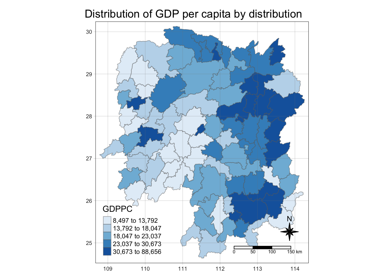
tmap_mode we set to “plot” to keep it static. We can easily change it to “view” to get an interactive map instead.
tm_field + tm_border will give you a polygon
6.0 Identify Neighbours Method
6.1 Contiguity Neighbours Method
In the code chunk below, st_contiguity() is used to derive a contiguity neighbour list by using Queen’s method.
https://sfdep.josiahparry.com/reference/st_contiguity.html for documentation
cn_queen <- hunan_GDPPC %>%
  mutate(nb = st_contiguity(geometry),
         .before = 1)

# nb is a list
# results will be stored as sf dataframe
# st_contiguity is performed on geometry column of hunan_GDPPC
# .before = 1 to put the newly created column before the first original column in hunan_GDPPC
Using the steps learned, derive a contiguity neighbour list using Rook’s method.
cn_queen will have 1 extra column more than hunan_GDPPC. You can see the corresponding neighbouring place under NAME_3 column in cn_queen.
cn_rook <- hunan_GDPPC %>%
  mutate(nb = st_contiguity(geometry),
         queen = FALSE,
         .before = 1)

# if you want to use bishop, must use spdep package instead. Normally, we do not use bishop method.
6.2 Computing Continguity Weights
6.2.1 Contiguity Weights: Queen’s method
wm_q <- hunan_GDPPC %>%
  mutate(nb = st_contiguity(geometry),
         wt = st_weights(nb),
         .before = 1)

# now I'll have 2 new columns nb and wt