pacman::p_load(sf, tidyverse, funModeling)Take-home Exercise 1
1.0 Overview
1.1 Background
Water is an important resource to mankind. Clean and accessible water is critical to human health. It provides a healthy environment, a sustainable economy, reduces poverty and ensures peace and security. Yet over 40% of the global population does not have access to sufficient clean water. By 2025, 1.8 billion people will be living in countries or regions with absolute water scarcity, according to UN-Water. The lack of water poses a major threat to several sectors, including food security. Agriculture uses about 70% of the world’s accessible freshwater.
Developing countries are most affected by water shortages and poor water quality. Up to 80% of illnesses in the developing world are linked to inadequate water and sanitation. Despite technological advancement, providing clean water to the rural community is still a major development issues in many countries globally, especially countries in the Africa continent.
To address the issue of providing clean and sustainable water supply to the rural community, a global Water Point Data Exchange (WPdx) project has been initiated. The main aim of this initiative is to collect water point related data from rural areas at the water point or small water scheme level and share the data via WPdx Data Repository, a cloud-based data library. What is so special of this project is that data are collected based on WPDx Data Standard.
1.2 Objectives/ Problem Statement
Geospatial analytics hold tremendous potential to address complex problems facing society. In this study, you are tasked to apply appropriate geospatial data wrangling methods to prepare the data for water point mapping study. For the purpose of this study, Nigeria will be used as the study country.
2.0 Setup
2.1 Packages Used
sf –> a relatively new R package specially designed to import, manage and process vector-based geospatial data in R.
tidyverse –> used for wrangling and visualisations
funModelling –> for EDA and visualisations
spatstat –> has a wide range of useful functions for point pattern analysis. Used to perform 1st- and 2nd-order spatial point patterns analysis and derive kernel density estimation (KDE) layer.
raster –> reads, writes, manipulates, analyses and model of gridded spatial data (i.e. raster)
tmap –> provides functions for plotting cartographic quality static point patterns maps or interactive maps by using leaflet API.
maptools –> provides a set of tools for manipulating geographic data. To convert Spatial objects into ppp format of spatstat.
sfdep –> simple feature spatial dependence
3.0 Importing Data
3.1 Importing Geospatial Data
geoNGA <- st_read("data/geospatial/",
layer = "geoBoundaries-NGA-ADM2") %>%
st_transform(crs = 26392)Reading layer `geoBoundaries-NGA-ADM2' from data source
`/Users/yashica/Desktop/xtc0/IS415-GAA/Take-home_Ex/Take_home_Ex01/data/geospatial'
using driver `ESRI Shapefile'
Simple feature collection with 774 features and 5 fields
Geometry type: MULTIPOLYGON
Dimension: XY
Bounding box: xmin: 2.668534 ymin: 4.273007 xmax: 14.67882 ymax: 13.89442
Geodetic CRS: WGS 84NGA <- st_read("data/geospatial/",
layer = "nga_admbnda_adm2_osgof_20190417") %>%
st_transform(crs = 26392)Reading layer `nga_admbnda_adm2_osgof_20190417' from data source
`/Users/yashica/Desktop/xtc0/IS415-GAA/Take-home_Ex/Take_home_Ex01/data/geospatial'
using driver `ESRI Shapefile'
Simple feature collection with 774 features and 16 fields
Geometry type: MULTIPOLYGON
Dimension: XY
Bounding box: xmin: 2.668534 ymin: 4.273007 xmax: 14.67882 ymax: 13.89442
Geodetic CRS: WGS 84Now, we’ll be looking at Osun State in Nigeria for our analysis.
osunNGA <- NGA %>% filter(NGA$ADM1_EN == "Osun")
osunNGASimple feature collection with 30 features and 16 fields
Geometry type: MULTIPOLYGON
Dimension: XY
Bounding box: xmin: 176503.2 ymin: 331434.7 xmax: 291043.8 ymax: 454520.1
Projected CRS: Minna / Nigeria Mid Belt
First 10 features:
Shape_Leng Shape_Area ADM2_EN ADM2_PCODE ADM2_REF ADM2ALT1EN
1 1.7951405 0.062436080 Aiyedade NG030001 Aiyedade <NA>
2 0.7101503 0.024818478 Aiyedire NG030002 Aiyedire <NA>
3 0.9199564 0.038002894 Atakumosa East NG030003 Atakumosa East <NA>
4 0.8502782 0.030445804 Atakumosa West NG030004 Atakumosa West <NA>
5 0.5212768 0.012213340 Boluwaduro NG030005 Boluwaduro <NA>
6 0.6088930 0.011827501 Boripe NG030006 Boripe <NA>
7 0.4714403 0.008343638 Ede North NG030007 Ede North <NA>
8 0.5660235 0.017623677 Ede South NG030008 Ede South <NA>
9 0.8273123 0.022026327 Egbedore NG030009 Egbedore <NA>
10 1.1304849 0.029791275 Ejigbo NG030010 Ejigbo <NA>
ADM2ALT2EN ADM1_EN ADM1_PCODE ADM0_EN ADM0_PCODE date validOn
1 <NA> Osun NG030 Nigeria NG 2016-11-29 2019-04-17
2 <NA> Osun NG030 Nigeria NG 2016-11-29 2019-04-17
3 <NA> Osun NG030 Nigeria NG 2016-11-29 2019-04-17
4 <NA> Osun NG030 Nigeria NG 2016-11-29 2019-04-17
5 <NA> Osun NG030 Nigeria NG 2016-11-29 2019-04-17
6 <NA> Osun NG030 Nigeria NG 2016-11-29 2019-04-17
7 <NA> Osun NG030 Nigeria NG 2016-11-29 2019-04-17
8 <NA> Osun NG030 Nigeria NG 2016-11-29 2019-04-17
9 <NA> Osun NG030 Nigeria NG 2016-11-29 2019-04-17
10 <NA> Osun NG030 Nigeria NG 2016-11-29 2019-04-17
validTo SD_EN SD_PCODE geometry
1 <NA> Osun West NG03003 MULTIPOLYGON (((213526.6 34...
2 <NA> Osun West NG03003 MULTIPOLYGON (((212542.6 40...
3 <NA> Osun East NG03002 MULTIPOLYGON (((265746.8 37...
4 <NA> Osun East NG03002 MULTIPOLYGON (((248871.4 40...
5 <NA> Osun Central NG03001 MULTIPOLYGON (((266092.2 43...
6 <NA> Osun Central NG03001 MULTIPOLYGON (((255072.5 43...
7 <NA> Osun West NG03003 MULTIPOLYGON (((236386.9 41...
8 <NA> Osun West NG03003 MULTIPOLYGON (((236386.9 41...
9 <NA> Osun West NG03003 MULTIPOLYGON (((220756 4317...
10 <NA> Osun West NG03003 MULTIPOLYGON (((214422.1 42...3.2 Importing Aspatial Data
3.2.1 Filtering Aspatial Data
wp_nga <- read_csv("data/aspatial/WPdx.csv") %>%
filter(`#clean_country_name` == "Nigeria") %>%
filter(`#clean_adm1` == "Osun")3.2.2 Converting Aspatial Data Into Geospatial
wp_nga$Geometry = st_as_sfc(wp_nga$`New Georeferenced Column`)
wp_nga# A tibble: 5,557 × 71
row_id `#source` #lat_…¹ #lon_…² #repo…³ #stat…⁴ #wate…⁵ #wate…⁶ #wate…⁷
<dbl> <chr> <dbl> <dbl> <chr> <chr> <chr> <chr> <chr>
1 429123 GRID3 8.02 5.06 08/29/… Unknown <NA> <NA> Tapsta…
2 70566 Federal Minis… 7.32 4.79 05/11/… No Protec… Well Mechan…
3 70578 Federal Minis… 7.76 4.56 05/11/… No Boreho… Well Mechan…
4 66401 Federal Minis… 8.03 4.64 04/30/… No Boreho… Well Mechan…
5 422190 GRID3 7.87 4.88 08/29/… Unknown <NA> <NA> Tapsta…
6 422064 GRID3 7.7 4.89 08/29/… Unknown <NA> <NA> Tapsta…
7 65607 Federal Minis… 7.89 4.71 05/12/… No Boreho… Well Mechan…
8 68989 Federal Minis… 7.51 4.27 05/07/… No Boreho… Well <NA>
9 67708 Federal Minis… 7.48 4.35 04/29/… Yes Boreho… Well Mechan…
10 66419 Federal Minis… 7.63 4.50 05/08/… Yes Boreho… Well Hand P…
# … with 5,547 more rows, 62 more variables: `#water_tech_category` <chr>,
# `#facility_type` <chr>, `#clean_country_name` <chr>, `#clean_adm1` <chr>,
# `#clean_adm2` <chr>, `#clean_adm3` <chr>, `#clean_adm4` <chr>,
# `#install_year` <dbl>, `#installer` <chr>, `#rehab_year` <lgl>,
# `#rehabilitator` <lgl>, `#management_clean` <chr>, `#status_clean` <chr>,
# `#pay` <chr>, `#fecal_coliform_presence` <chr>,
# `#fecal_coliform_value` <dbl>, `#subjective_quality` <chr>, …wp_sf <- st_sf(wp_nga, crs=4326)
wp_sfSimple feature collection with 5557 features and 70 fields
Geometry type: POINT
Dimension: XY
Bounding box: xmin: 4.032004 ymin: 7.060309 xmax: 5.06 ymax: 8.061898
Geodetic CRS: WGS 84
# A tibble: 5,557 × 71
row_id `#source` #lat_…¹ #lon_…² #repo…³ #stat…⁴ #wate…⁵ #wate…⁶ #wate…⁷
* <dbl> <chr> <dbl> <dbl> <chr> <chr> <chr> <chr> <chr>
1 429123 GRID3 8.02 5.06 08/29/… Unknown <NA> <NA> Tapsta…
2 70566 Federal Minis… 7.32 4.79 05/11/… No Protec… Well Mechan…
3 70578 Federal Minis… 7.76 4.56 05/11/… No Boreho… Well Mechan…
4 66401 Federal Minis… 8.03 4.64 04/30/… No Boreho… Well Mechan…
5 422190 GRID3 7.87 4.88 08/29/… Unknown <NA> <NA> Tapsta…
6 422064 GRID3 7.7 4.89 08/29/… Unknown <NA> <NA> Tapsta…
7 65607 Federal Minis… 7.89 4.71 05/12/… No Boreho… Well Mechan…
8 68989 Federal Minis… 7.51 4.27 05/07/… No Boreho… Well <NA>
9 67708 Federal Minis… 7.48 4.35 04/29/… Yes Boreho… Well Mechan…
10 66419 Federal Minis… 7.63 4.50 05/08/… Yes Boreho… Well Hand P…
# … with 5,547 more rows, 62 more variables: `#water_tech_category` <chr>,
# `#facility_type` <chr>, `#clean_country_name` <chr>, `#clean_adm1` <chr>,
# `#clean_adm2` <chr>, `#clean_adm3` <chr>, `#clean_adm4` <chr>,
# `#install_year` <dbl>, `#installer` <chr>, `#rehab_year` <lgl>,
# `#rehabilitator` <lgl>, `#management_clean` <chr>, `#status_clean` <chr>,
# `#pay` <chr>, `#fecal_coliform_presence` <chr>,
# `#fecal_coliform_value` <dbl>, `#subjective_quality` <chr>, …wp_sf <- wp_sf %>%
st_transform(crs = 26392)wp_sf <- wp_sf %>%
filter(`#clean_country_name` == "Nigeria") %>%
filter(`#clean_adm1` == "Osun")4.0 Geospatial Data Cleaning
Data cleaning is an important step in any data science task including geospatial data science. It is important for us to do our due diligence to check if any data quality issues occured in the data used.
4.1 Excluding Redundant Fields
Looking through the osunNGA dataframe, we can conclude that there are NO redundant fields.
4.2 Checking For Duplicate Values In Columns
It is always important to check for duplicate name in the data main data fields. Using duplicated() of Base R, we can flag out duplicates.
osunNGA$ADM2_EN[duplicated(osunNGA$ADM2_EN)==TRUE]character(0)Great! There are no duplicate values in the column “ADM2_EN”.
5.0 Data Wrangling For Water Point Data
Exploratory Data Analysis (EDA) is a popular approach to gain initial understanding of the data. In the code chunk below, freq() of funModeling package is used to reveal the distribution of water point status visually.
freq(data = wp_sf,
input = '#status_clean')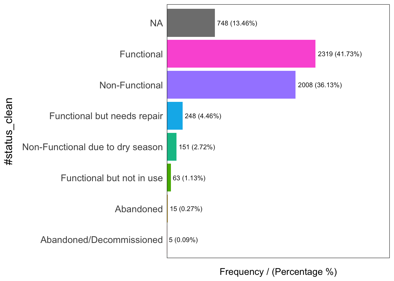
#status_clean frequency percentage cumulative_perc
1 Functional 2319 41.73 41.73
2 Non-Functional 2008 36.13 77.86
3 <NA> 748 13.46 91.32
4 Functional but needs repair 248 4.46 95.78
5 Non-Functional due to dry season 151 2.72 98.50
6 Functional but not in use 63 1.13 99.63
7 Abandoned 15 0.27 99.90
8 Abandoned/Decommissioned 5 0.09 100.00Figure above shows that there are nine classes in the #status_clean fields.
Next, code chunk below will be used to perform the following data wrangling tasksP - rename() of dplyr package is used to rename the column from #status_clean to status_clean for easier handling in subsequent steps. - select() of dplyr is used to include status_clean in the output sf data.frame. - mutate() and replace_na() are used to recode all the NA values in status_clean into unknown.
wp_sf_nga <- wp_sf %>%
rename(status_clean = '#status_clean') %>%
select(status_clean) %>%
mutate(status_clean = replace_na(
status_clean, "unknown"))wp_sf_ngaSimple feature collection with 5557 features and 1 field
Geometry type: POINT
Dimension: XY
Bounding box: xmin: 177285.9 ymin: 340054.1 xmax: 291287.1 ymax: 450859.7
Projected CRS: Minna / Nigeria Mid Belt
# A tibble: 5,557 × 2
status_clean Geometry
* <chr> <POINT [m]>
1 unknown (291287.1 445959)
2 Abandoned/Decommissioned (260303.8 368418.2)
3 Abandoned/Decommissioned (236239.7 417577)
4 Abandoned/Decommissioned (244631.9 447614.1)
5 unknown (271267.3 429512.8)
6 unknown (272211 410670.5)
7 Abandoned/Decommissioned (252887.8 432017.8)
8 Abandoned/Decommissioned (202912.5 390196.1)
9 Functional but needs repair (212810 386707.6)
10 Functional (228798.9 403822.5)
# … with 5,547 more rows5.1 Extracting Water Point Data
This code chunk below extracts functional water points.
wp_functional <- wp_sf_nga %>%
filter(status_clean %in%
c("Functional",
"Functional but not in use",
"Functional but needs repair"))This code chunk below extracts non-functional water points.
wp_nonfunctional <- wp_sf_nga %>%
filter(status_clean %in%
c("Abandoned/Decommissioned",
"Abandoned",
"Non-Functional due to dry season",
"Non-Functional",
"Non functional due to dry season"))The code chunk below is used to extract water point with unknown status.
wp_unknown <- wp_sf_nga %>%
filter(status_clean == "unknown")Next, the code chunk below is used to perform a quick EDA on the derived sf data.frames.
freq(data = wp_functional,
input = 'status_clean')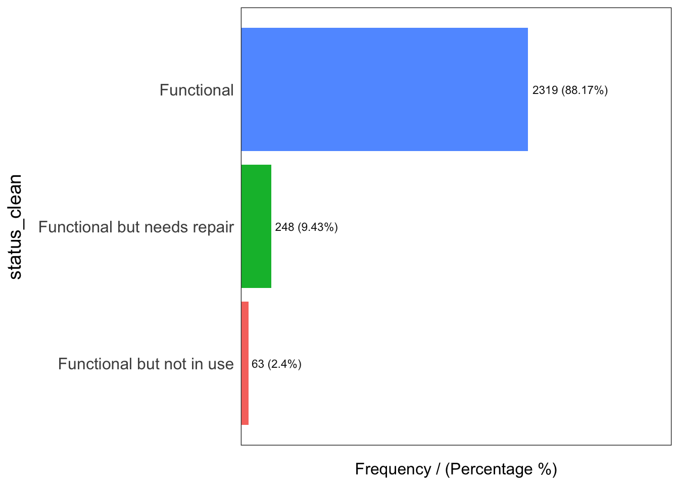
status_clean frequency percentage cumulative_perc
1 Functional 2319 88.17 88.17
2 Functional but needs repair 248 9.43 97.60
3 Functional but not in use 63 2.40 100.00freq(data = wp_nonfunctional,
input = 'status_clean')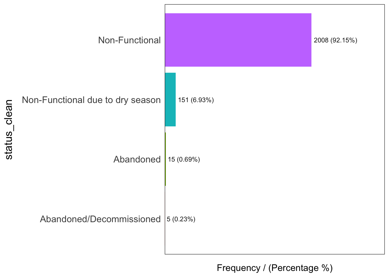
status_clean frequency percentage cumulative_perc
1 Non-Functional 2008 92.15 92.15
2 Non-Functional due to dry season 151 6.93 99.08
3 Abandoned 15 0.69 99.77
4 Abandoned/Decommissioned 5 0.23 100.00freq(data = wp_unknown,
input = 'status_clean')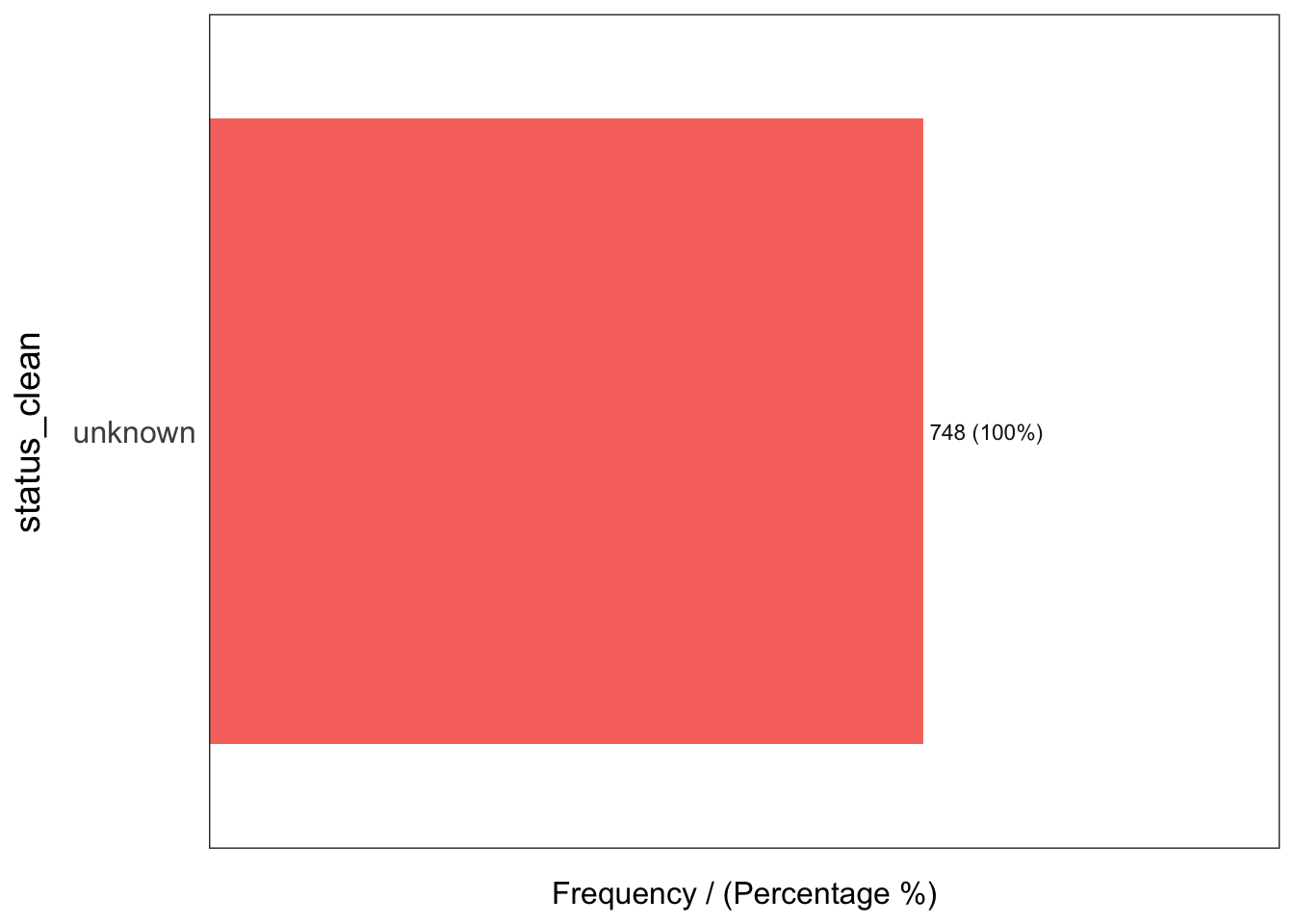
status_clean frequency percentage cumulative_perc
1 unknown 748 100 1006.0 Mapping Geospatial Datasets
Now, we’re importing more packages to create maps for visualisations.
pacman::p_load(maptools, raster, spatstat, tmap)tmap_mode('view')
tm_shape(wp_sf_nga)+
tm_dots()tmap_mode('plot')7.0 Geospatial Data Wrangling
7.1 Converting sf Dataframes to sp’s Spatial Class
wp_functionalSimple feature collection with 2630 features and 1 field
Geometry type: POINT
Dimension: XY
Bounding box: xmin: 177285.9 ymin: 343128.1 xmax: 290751 ymax: 450859.7
Projected CRS: Minna / Nigeria Mid Belt
# A tibble: 2,630 × 2
status_clean Geometry
* <chr> <POINT [m]>
1 Functional but needs repair (212810 386707.6)
2 Functional (228798.9 403822.5)
3 Functional (270497.9 377476.9)
4 Functional (212202 349210.1)
5 Functional (259331.9 399591.4)
6 Functional (195484 404733.2)
7 Functional (221302.3 389473.6)
8 Functional but not in use (263254.1 382692.9)
9 Functional (192484.1 405113)
10 Functional (252736 373593)
# … with 2,620 more rowswp_nonfunctionalSimple feature collection with 2179 features and 1 field
Geometry type: POINT
Dimension: XY
Bounding box: xmin: 180539 ymin: 340054.1 xmax: 290616 ymax: 450780.1
Projected CRS: Minna / Nigeria Mid Belt
# A tibble: 2,179 × 2
status_clean Geometry
* <chr> <POINT [m]>
1 Abandoned/Decommissioned (260303.8 368418.2)
2 Abandoned/Decommissioned (236239.7 417577)
3 Abandoned/Decommissioned (244631.9 447614.1)
4 Abandoned/Decommissioned (252887.8 432017.8)
5 Abandoned/Decommissioned (202912.5 390196.1)
6 Abandoned (203615.2 438277.3)
7 Abandoned (255213.6 401175.9)
8 Abandoned (255869 398845.1)
9 Abandoned (254321.8 437453)
10 Abandoned (201613.1 436132.1)
# … with 2,169 more rowsThe code chunk below uses as_Spatial() of sf package to convert the three geospatial data from simple feature data frame to sp’s Spatial* class.
wp_functional_spatial <- as_Spatial(wp_functional)
wp_nonfunctional_spatial <- as_Spatial(wp_nonfunctional)
osunNGA_spatial <- as_Spatial(osunNGA)wp_functional_spatialclass : SpatialPointsDataFrame
features : 2630
extent : 177285.9, 290751, 343128.1, 450859.7 (xmin, xmax, ymin, ymax)
crs : +proj=tmerc +lat_0=4 +lon_0=8.5 +k=0.99975 +x_0=670553.98 +y_0=0 +a=6378249.145 +rf=293.465 +towgs84=-92,-93,122,0,0,0,0 +units=m +no_defs
variables : 1
names : status_clean
min values : Functional
max values : Functional but not in use wp_nonfunctional_spatialclass : SpatialPointsDataFrame
features : 2179
extent : 180539, 290616, 340054.1, 450780.1 (xmin, xmax, ymin, ymax)
crs : +proj=tmerc +lat_0=4 +lon_0=8.5 +k=0.99975 +x_0=670553.98 +y_0=0 +a=6378249.145 +rf=293.465 +towgs84=-92,-93,122,0,0,0,0 +units=m +no_defs
variables : 1
names : status_clean
min values : Abandoned
max values : Non-Functional due to dry season osunNGA_spatialclass : SpatialPolygonsDataFrame
features : 30
extent : 176503.2, 291043.8, 331434.7, 454520.1 (xmin, xmax, ymin, ymax)
crs : +proj=tmerc +lat_0=4 +lon_0=8.5 +k=0.99975 +x_0=670553.98 +y_0=0 +a=6378249.145 +rf=293.465 +towgs84=-92,-93,122,0,0,0,0 +units=m +no_defs
variables : 16
names : Shape_Leng, Shape_Area, ADM2_EN, ADM2_PCODE, ADM2_REF, ADM2ALT1EN, ADM2ALT2EN, ADM1_EN, ADM1_PCODE, ADM0_EN, ADM0_PCODE, date, validOn, validTo, SD_EN, ...
min values : 0.26445678806, 0.00248649736648, Aiyedade, NG030001, Aiyedade, NA, NA, Osun, NG030, Nigeria, NG, 17134, 18003, NA, Osun Central, ...
max values : 1.8470166597, 0.0737271661922, Osogbo, NG030030, Osogbo, NA, NA, Osun, NG030, Nigeria, NG, 17134, 18003, NA, Osun West, ... 7.2 Converting the Spatial* class into generic sp format
spatstat requires the analytical data in ppp object form. There is no direct way to convert a Spatial* classes into ppp object. We need to convert the Spatial classes* into Spatial object first. The codes chunk below converts the Spatial* classes into generic sp objects.
wp_functional_spatial_sp <- as(wp_functional_spatial, "SpatialPoints")
wp_nonfunctional_spatial_sp <- as(wp_nonfunctional_spatial, "SpatialPoints")
osunNGA_spatial_sp <- as(osunNGA_spatial, "SpatialPolygons")Next, you should display the sp objects properties as shown below.
wp_functional_spatial_spclass : SpatialPoints
features : 2630
extent : 177285.9, 290751, 343128.1, 450859.7 (xmin, xmax, ymin, ymax)
crs : +proj=tmerc +lat_0=4 +lon_0=8.5 +k=0.99975 +x_0=670553.98 +y_0=0 +a=6378249.145 +rf=293.465 +towgs84=-92,-93,122,0,0,0,0 +units=m +no_defs wp_nonfunctional_spatial_spclass : SpatialPoints
features : 2179
extent : 180539, 290616, 340054.1, 450780.1 (xmin, xmax, ymin, ymax)
crs : +proj=tmerc +lat_0=4 +lon_0=8.5 +k=0.99975 +x_0=670553.98 +y_0=0 +a=6378249.145 +rf=293.465 +towgs84=-92,-93,122,0,0,0,0 +units=m +no_defs osunNGA_spatial_spclass : SpatialPolygons
features : 30
extent : 176503.2, 291043.8, 331434.7, 454520.1 (xmin, xmax, ymin, ymax)
crs : +proj=tmerc +lat_0=4 +lon_0=8.5 +k=0.99975 +x_0=670553.98 +y_0=0 +a=6378249.145 +rf=293.465 +towgs84=-92,-93,122,0,0,0,0 +units=m +no_defs 7.3 Converting the generic sp format into spatstat’s ppp format
Now, we will use as.ppp() function of spatstat to convert the spatial data into spatstat’s ppp object format.
wp_functional_spatial_ppp <- as(wp_functional_spatial_sp, "ppp")
wp_functional_spatial_pppPlanar point pattern: 2630 points
window: rectangle = [177285.9, 290750.96] x [343128.1, 450859.7] unitswp_nonfunctional_spatial_ppp <- as(wp_nonfunctional_spatial_sp, "ppp")
wp_nonfunctional_spatial_pppPlanar point pattern: 2179 points
window: rectangle = [180538.96, 290616] x [340054.1, 450780.1] unitsLet us plot wp_functional_spatial_ppp and examine the difference.
plot(wp_functional_spatial_ppp)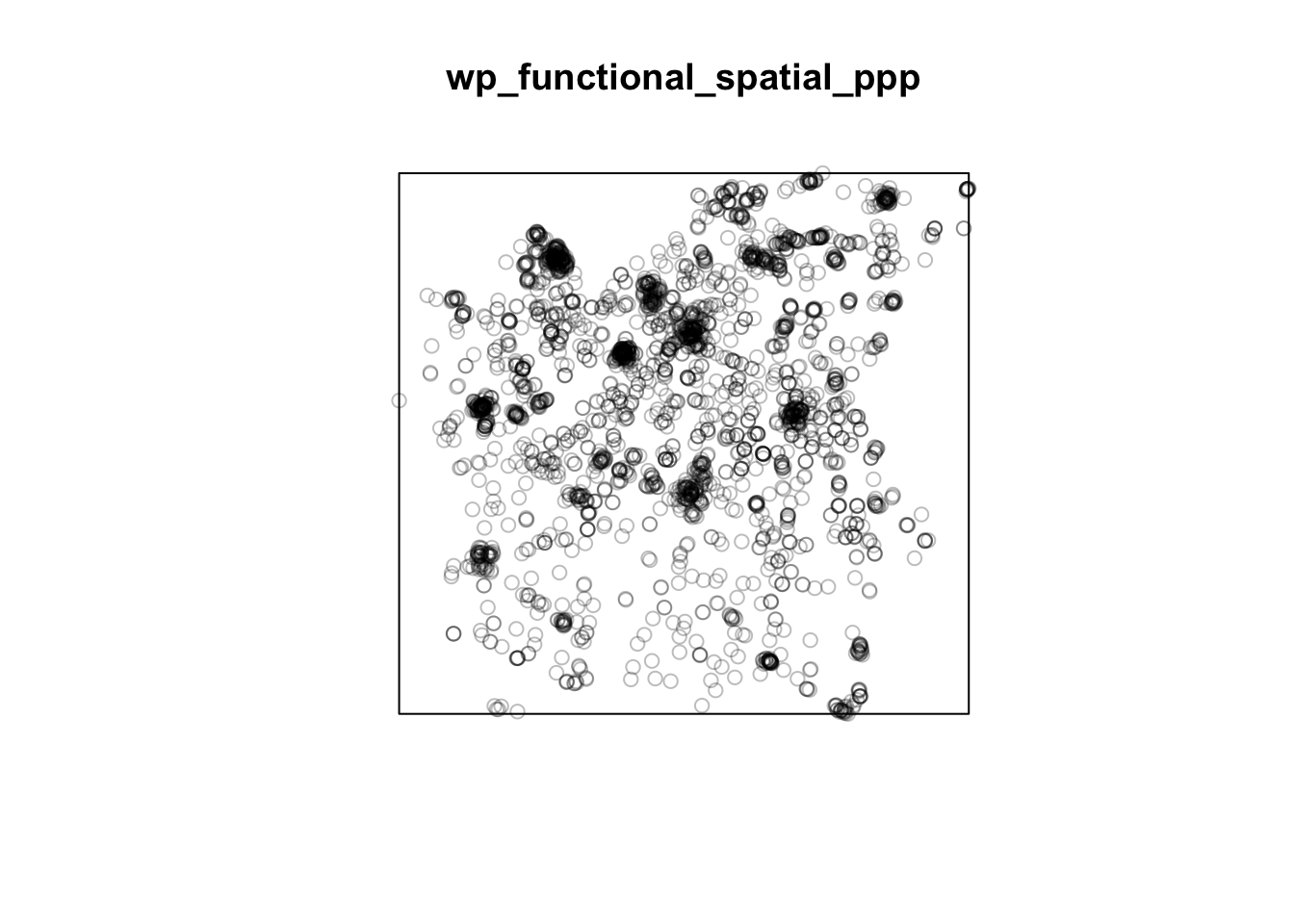
Now, let’s plot wp_nonfunctional_spatial_ppp.
plot(wp_nonfunctional_spatial_ppp)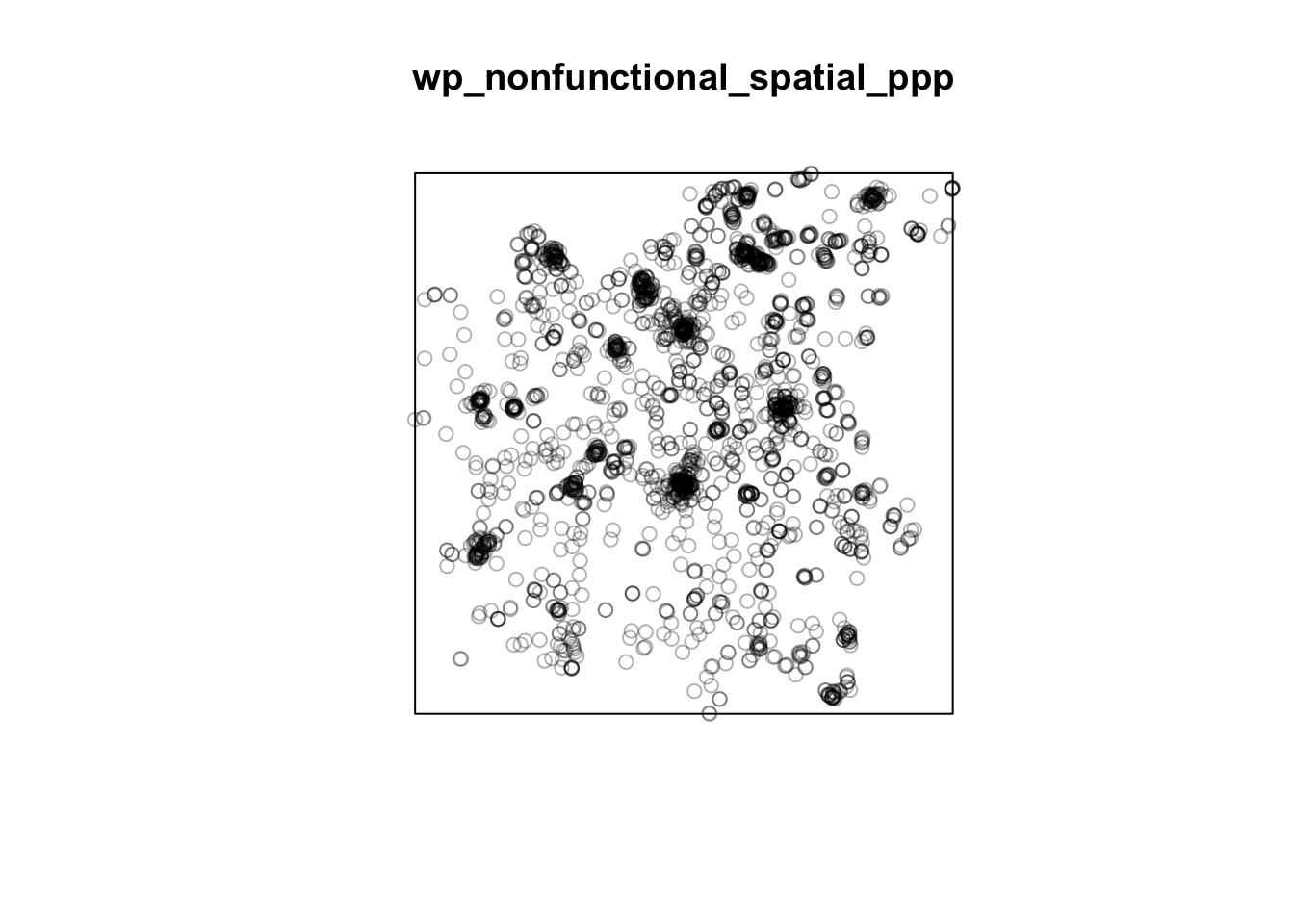
You can take a quick look at the summary statistics of the newly created ppp objects by using the code chunk below.
summary(wp_functional_spatial_ppp)Planar point pattern: 2630 points
Average intensity 2.151545e-07 points per square unit
Coordinates are given to 2 decimal places
i.e. rounded to the nearest multiple of 0.01 units
Window: rectangle = [177285.9, 290750.96] x [343128.1, 450859.7] units
(113500 x 107700 units)
Window area = 12223800000 square unitssummary(wp_nonfunctional_spatial_ppp)Planar point pattern: 2179 points
Average intensity 1.787766e-07 points per square unit
Coordinates are given to 2 decimal places
i.e. rounded to the nearest multiple of 0.01 units
Window: rectangle = [180538.96, 290616] x [340054.1, 450780.1] units
(110100 x 110700 units)
Window area = 12188400000 square units7.4 Handling Duplicated Points
Now, we’ll be checking for duplicates in both wp_functional_spatial_ppp and wp_nonfunctional_spatial_ppp objects. If duplicates are found, further processing is required.
any(duplicated(wp_functional_spatial_ppp))[1] FALSEany(duplicated(wp_nonfunctional_spatial_ppp))[1] FALSEGreat! No duplicates are found for both wp_functional_spatial_ppp and wp_nonfunctional_spatial_ppp objects!
7.5 Creating owin Object
When analysing spatial point patterns, it is a good practice to confine the analysis with a geographical area like Osun State boundary. In spatstat, an object called owin is specially designed to represent this polygonal region.
The code chunk below is used to covert sg SpatialPolygon object into owin object of spatstat.
osun_owin <- as(osunNGA_spatial_sp, "owin")plot(osun_owin)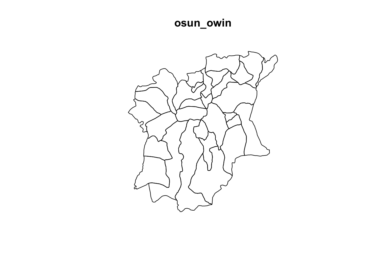
summary(osun_owin)Window: polygonal boundary
30 separate polygons (no holes)
vertices area relative.area
polygon 1 204 766084000 0.08870
polygon 2 81 304399000 0.03520
polygon 3 97 465688000 0.05390
polygon 4 124 373051000 0.04320
polygon 5 60 149473000 0.01730
polygon 6 84 144820000 0.01680
polygon 7 50 102243000 0.01180
polygon 8 72 216002000 0.02500
polygon 9 112 269897000 0.03130
polygon 10 125 365142000 0.04230
polygon 11 83 111191000 0.01290
polygon 12 126 192557000 0.02230
polygon 13 219 904397000 0.10500
polygon 14 174 741131000 0.08580
polygon 15 81 138742000 0.01610
polygon 16 65 119452000 0.01380
polygon 17 90 280205000 0.03240
polygon 18 69 69814600 0.00808
polygon 19 69 42727500 0.00495
polygon 20 49 30458800 0.00353
polygon 21 62 263505000 0.03050
polygon 22 93 438930000 0.05080
polygon 23 87 274127000 0.03170
polygon 24 105 509979000 0.05910
polygon 25 98 292058000 0.03380
polygon 26 64 327765000 0.03800
polygon 27 133 108945000 0.01260
polygon 28 122 462169000 0.05350
polygon 29 94 109715000 0.01270
polygon 30 95 61239800 0.00709
enclosing rectangle: [176503.22, 291043.82] x [331434.7, 454520.1] units
(114500 x 123100 units)
Window area = 8635910000 square units
Fraction of frame area: 0.6137.6 Combining Point Events Object and Owin Object
First, let’s combine wp_functional_spatial_ppp points with osun_owin.
wp_functional_osun_ppp = wp_functional_spatial_ppp[osun_owin]summary(wp_functional_osun_ppp)Planar point pattern: 2529 points
Average intensity 2.928471e-07 points per square unit
Coordinates are given to 2 decimal places
i.e. rounded to the nearest multiple of 0.01 units
Window: polygonal boundary
30 separate polygons (no holes)
vertices area relative.area
polygon 1 204 766084000 0.08870
polygon 2 81 304399000 0.03520
polygon 3 97 465688000 0.05390
polygon 4 124 373051000 0.04320
polygon 5 60 149473000 0.01730
polygon 6 84 144820000 0.01680
polygon 7 50 102243000 0.01180
polygon 8 72 216002000 0.02500
polygon 9 112 269897000 0.03130
polygon 10 125 365142000 0.04230
polygon 11 83 111191000 0.01290
polygon 12 126 192557000 0.02230
polygon 13 219 904397000 0.10500
polygon 14 174 741131000 0.08580
polygon 15 81 138742000 0.01610
polygon 16 65 119452000 0.01380
polygon 17 90 280205000 0.03240
polygon 18 69 69814600 0.00808
polygon 19 69 42727500 0.00495
polygon 20 49 30458800 0.00353
polygon 21 62 263505000 0.03050
polygon 22 93 438930000 0.05080
polygon 23 87 274127000 0.03170
polygon 24 105 509979000 0.05910
polygon 25 98 292058000 0.03380
polygon 26 64 327765000 0.03800
polygon 27 133 108945000 0.01260
polygon 28 122 462169000 0.05350
polygon 29 94 109715000 0.01270
polygon 30 95 61239800 0.00709
enclosing rectangle: [176503.22, 291043.82] x [331434.7, 454520.1] units
(114500 x 123100 units)
Window area = 8635910000 square units
Fraction of frame area: 0.613Now, let’s combine wp_nonfunctional_spatial_ppp points with osun_owin.
wp_nonfunctional_osun_ppp = wp_nonfunctional_spatial_ppp[osun_owin]summary(wp_nonfunctional_osun_ppp)Planar point pattern: 2059 points
Average intensity 2.384232e-07 points per square unit
Coordinates are given to 2 decimal places
i.e. rounded to the nearest multiple of 0.01 units
Window: polygonal boundary
30 separate polygons (no holes)
vertices area relative.area
polygon 1 204 766084000 0.08870
polygon 2 81 304399000 0.03520
polygon 3 97 465688000 0.05390
polygon 4 124 373051000 0.04320
polygon 5 60 149473000 0.01730
polygon 6 84 144820000 0.01680
polygon 7 50 102243000 0.01180
polygon 8 72 216002000 0.02500
polygon 9 112 269897000 0.03130
polygon 10 125 365142000 0.04230
polygon 11 83 111191000 0.01290
polygon 12 126 192557000 0.02230
polygon 13 219 904397000 0.10500
polygon 14 174 741131000 0.08580
polygon 15 81 138742000 0.01610
polygon 16 65 119452000 0.01380
polygon 17 90 280205000 0.03240
polygon 18 69 69814600 0.00808
polygon 19 69 42727500 0.00495
polygon 20 49 30458800 0.00353
polygon 21 62 263505000 0.03050
polygon 22 93 438930000 0.05080
polygon 23 87 274127000 0.03170
polygon 24 105 509979000 0.05910
polygon 25 98 292058000 0.03380
polygon 26 64 327765000 0.03800
polygon 27 133 108945000 0.01260
polygon 28 122 462169000 0.05350
polygon 29 94 109715000 0.01270
polygon 30 95 61239800 0.00709
enclosing rectangle: [176503.22, 291043.82] x [331434.7, 454520.1] units
(114500 x 123100 units)
Window area = 8635910000 square units
Fraction of frame area: 0.6138.0 First-order Spatial Point Patterns Analysis
In this section, we will perform first-order SPPA by using spatstat package. We will focus on:
- deriving kernel density estimation (KDE) layer for visualising and exploring the intensity of point processes,
8.1 Kernel Density Estimation
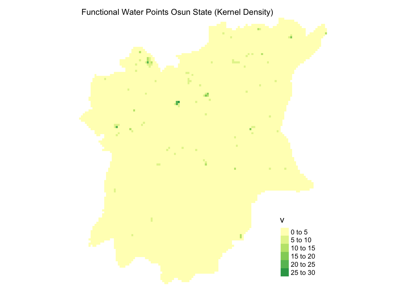
In this section, we will compute the kernel density estimation (KDE) of functional and non-functional waterpoints in Osun State.
8.1.1 Computing kernel density estimation using automatic bandwidth selection method
The code chunk below computes a kernel density by using the following configurations of density() of spatstat:
- bw.diggle() automatic bandwidth selection method. Other recommended methods are bw.CvL(), bw.scott() or bw.ppl().
We’re computing the kernel density for the functional waterpoints in Osun state.
kde_functional_osun_bw <- density(wp_functional_osun_ppp,
sigma=bw.diggle,
edge=TRUE,
kernel="gaussian") The plot() function of Base R is then used to display the kernel density derived.
plot(kde_functional_osun_bw)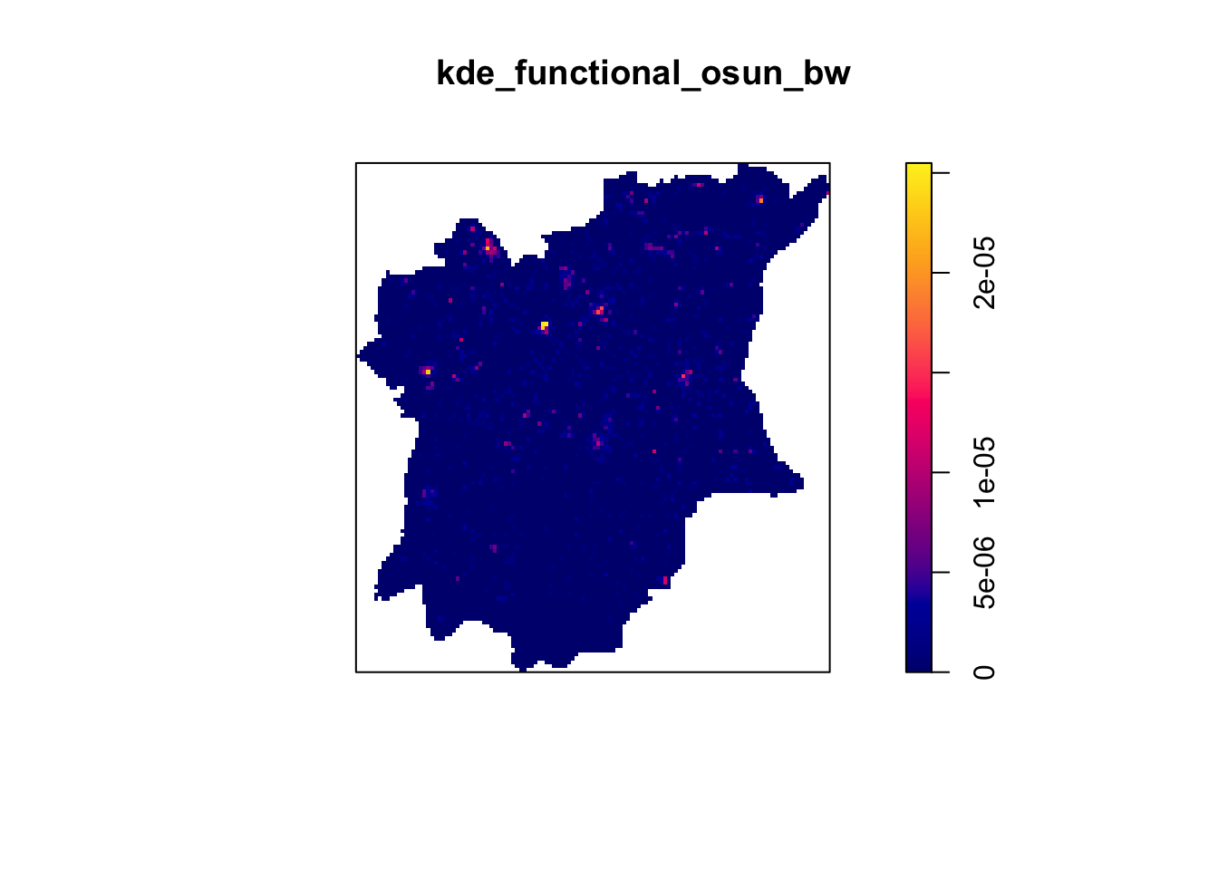
The density values of the output range is way too small to comprehend. This is because the default unit of measurement of svy21 is in meter. As a result, the density values computed is in “number of points per square meter”.
We’re now computing the kernel density for the non-functional waterpoints in Osun state.
kde_nonfunctional_osun_bw <- density(wp_nonfunctional_osun_ppp,
sigma=bw.diggle,
edge=TRUE,
kernel="gaussian") plot(kde_nonfunctional_osun_bw)
Before we move on to next section, it is good to know that you can retrieve the bandwidth used to compute the kde layer by using the code chunk below.
func_bw <- bw.diggle(wp_functional_osun_ppp)
func_bw sigma
252.1687 nonfunc_bw <- bw.diggle(wp_nonfunctional_osun_ppp)
nonfunc_bw sigma
308.2061 8.1.2 Rescalling KDE values
In the code chunk below, rescale() is used to covert the unit of measurement from meter to kilometer.
wp_functional_osun_ppp.km <- rescale(wp_functional_osun_ppp, 1000, "km")We’ll do rescaling for the functional waterpoints in Osun first.
kde_wp_functional_osun.bw <- density(wp_functional_osun_ppp.km, sigma=bw.diggle, edge=TRUE, kernel="gaussian")
plot(kde_wp_functional_osun.bw)
Notice that output image looks identical to the earlier version, the only changes in the data values (refer to the legend).
Now, we’ll do rescaling for the non-functional waterpoints in Osun.
wp_nonfunctional_osun_ppp.km <- rescale(wp_nonfunctional_osun_ppp, 1000, "km")kde_wp_nonfunctional_osun.bw <- density(wp_nonfunctional_osun_ppp.km, sigma=bw.diggle, edge=TRUE, kernel="gaussian")
plot(kde_wp_nonfunctional_osun.bw)
8.2 Fixed and Adaptive KDE
8.2.1 Computing KDE using Fixed Bandwidth
Next, we will compute a KDE layer by defining a bandwidth of 600 meter. Notice that in the code chunk below, the sigma value used is 0.6. This is because the unit of measurement of wp_functional_osun_ppp.km and wp_nonfunctional_osun_ppp.km objects is in kilometer, hence the 600m is 0.6km.
kde_wp_functional_osun_600 <- density(wp_functional_osun_ppp.km, sigma=0.6, edge=TRUE, kernel="gaussian")
plot(kde_wp_functional_osun_600)
kde_wp_nonfunctional_osun_600 <- density(wp_nonfunctional_osun_ppp.km, sigma=0.6, edge=TRUE, kernel="gaussian")
plot(kde_wp_nonfunctional_osun_600)
8.2.2 Computing KDE using Adaptive Bandwidth
Fixed bandwidth method is very sensitive to highly skewed distribution of spatial point patterns over geographical units for example urban versus rural. One way to overcome this problem is by using adaptive bandwidth instead.
In this section, we will learn to derive adaptive kernel density estimation by using density.adaptive() of spatstat.
kde_wp_functional_osun_adaptive <- adaptive.density(wp_functional_osun_ppp.km, method="kernel")
plot(kde_wp_functional_osun_adaptive)
kde_wp_nonfunctional_osun_adaptive <- adaptive.density(wp_nonfunctional_osun_ppp.km, method="kernel")
plot(kde_wp_nonfunctional_osun_adaptive)
We can compare the fixed and adaptive kernel density estimation outputs by using the code chunk below.
For functional waterpoints in Osun State:
par(mfrow=c(1,2))
plot(kde_wp_functional_osun.bw, main = "Fixed bandwidth Func")
plot(kde_wp_functional_osun_adaptive, main = "Adaptive bandwidth Func")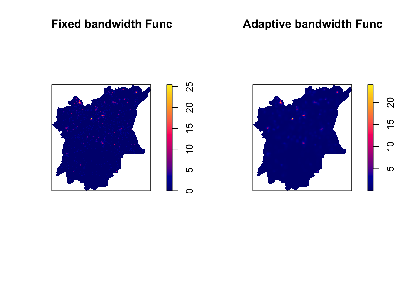
For nonfunctional waterpoints in Osun State:
par(mfrow=c(1,2))
plot(kde_wp_nonfunctional_osun.bw, main = "Fixed bandwidth NonFunc")
plot(kde_wp_nonfunctional_osun_adaptive, main = "Adaptive bandwidth NonFunc")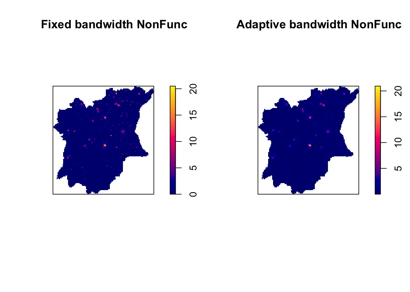
8.2.3 Converting KDE Output Into Grid Object
The result is the same, we just convert it so that it is suitable for mapping purposes.
gridded_kde_wp_functional_osun_bw <- as.SpatialGridDataFrame.im(kde_wp_functional_osun.bw)
spplot(gridded_kde_wp_functional_osun_bw)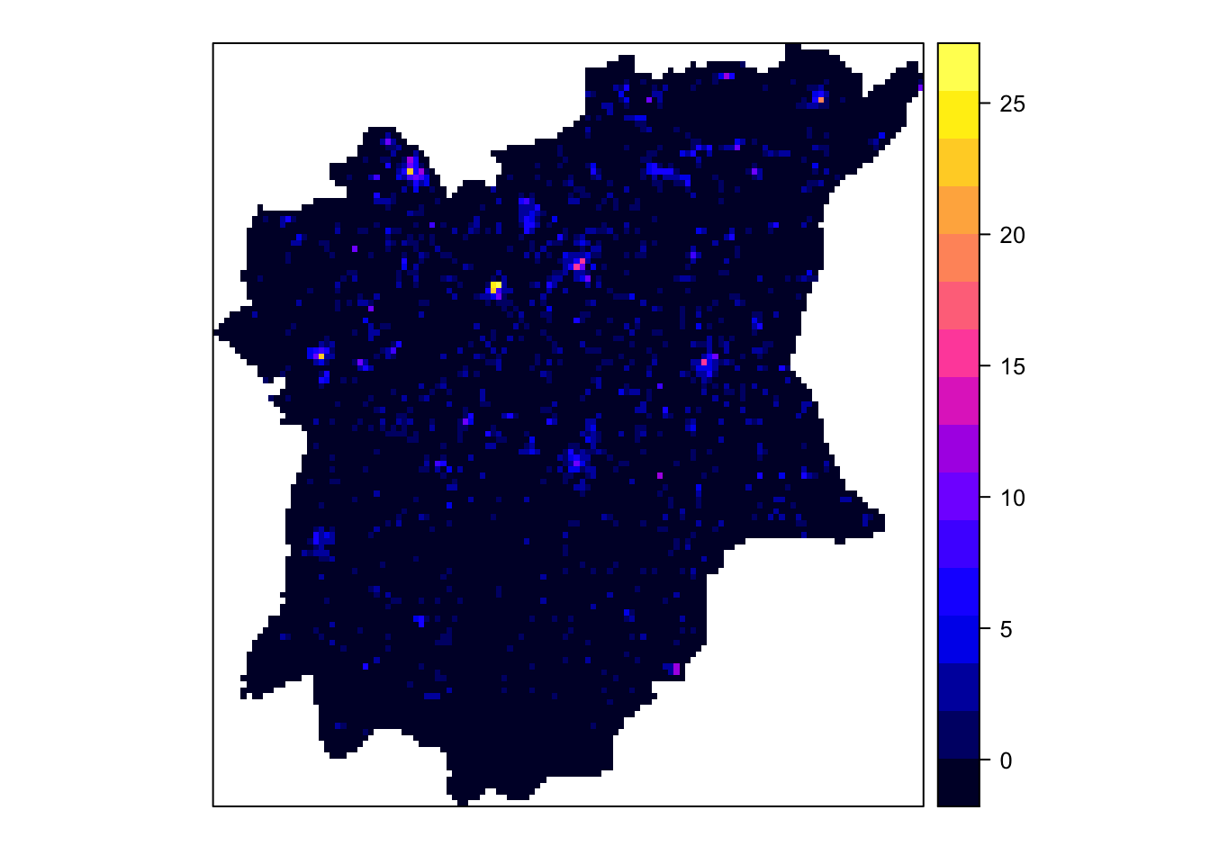
From the kernal density map generated by gridded_kde_wp_functional_osun_bw, we can tell that the regions with high number of functional water points usually cluster together in certain spots (in the Northern parts of Osun State). These regions are usually in pink, indicating that there are around 15 functional water points at each pink spot.
From the map, there’s only region which has an extremely high number of functional water points. This is highlighted by the yellow spots in the map.
From the map, we can conclude that the South of Osun State does not have many functional water points.
gridded_kde_wp_nonfunctional_osun_bw <- as.SpatialGridDataFrame.im(kde_wp_nonfunctional_osun.bw)
spplot(gridded_kde_wp_nonfunctional_osun_bw)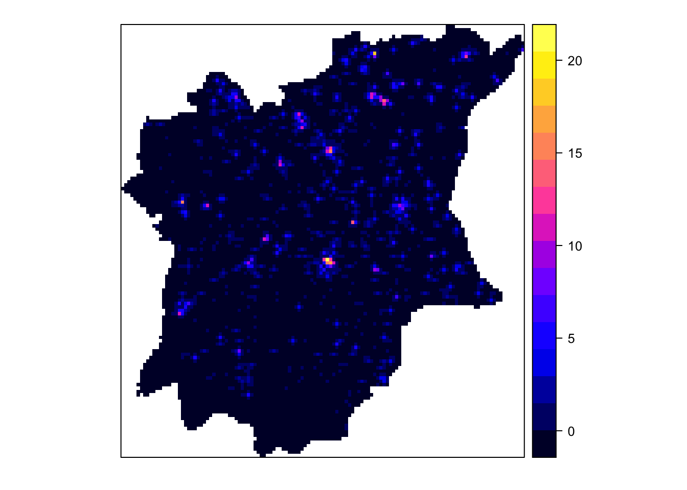
From the map generated by gridded_kde_wp_nonfunctional_osun_bw, we can tell that there are many non-functional water points in Osun State - even more than the functional water points. The regions with high concentrations (indicated by the pink spots) of non-functional water points tend to be at the centre to Northern parts of Osun State.
8.2.3.1 Converting Gridded Output into Raster
Next, we will convert the gridded kernal density objects into RasterLayer object by using raster() of raster package.
Functional waterpoints in Osun State
kde_wp_functional_bw_raster <- raster(gridded_kde_wp_functional_osun_bw)kde_wp_functional_bw_rasterclass : RasterLayer
dimensions : 128, 128, 16384 (nrow, ncol, ncell)
resolution : 0.8948485, 0.9616045 (x, y)
extent : 176.5032, 291.0438, 331.4347, 454.5201 (xmin, xmax, ymin, ymax)
crs : NA
source : memory
names : v
values : -4.569785e-15, 25.49435 (min, max)Non-functional waterpoints in Osun State
kde_wp_nonfunctional_bw_raster <- raster(gridded_kde_wp_nonfunctional_osun_bw)kde_wp_nonfunctional_bw_rasterclass : RasterLayer
dimensions : 128, 128, 16384 (nrow, ncol, ncell)
resolution : 0.8948485, 0.9616045 (x, y)
extent : 176.5032, 291.0438, 331.4347, 454.5201 (xmin, xmax, ymin, ymax)
crs : NA
source : memory
names : v
values : -3.965311e-15, 20.49412 (min, max)8.2.3.2 Assigning Projection Systems
The code chunk below will be used to include the CRS information on kde_wp_functional_bw_raster RasterLayer.
projection(kde_wp_functional_bw_raster) <- CRS("+init=EPSG:3414")
kde_wp_functional_bw_rasterclass : RasterLayer
dimensions : 128, 128, 16384 (nrow, ncol, ncell)
resolution : 0.8948485, 0.9616045 (x, y)
extent : 176.5032, 291.0438, 331.4347, 454.5201 (xmin, xmax, ymin, ymax)
crs : +init=EPSG:3414
source : memory
names : v
values : -4.569785e-15, 25.49435 (min, max)The code chunk below will be used to include the CRS information on kde_wp_nonfunctional_bw_raster RasterLayer.
projection(kde_wp_nonfunctional_bw_raster) <- CRS("+init=EPSG:3414")
kde_wp_nonfunctional_bw_rasterclass : RasterLayer
dimensions : 128, 128, 16384 (nrow, ncol, ncell)
resolution : 0.8948485, 0.9616045 (x, y)
extent : 176.5032, 291.0438, 331.4347, 454.5201 (xmin, xmax, ymin, ymax)
crs : +init=EPSG:3414
source : memory
names : v
values : -3.965311e-15, 20.49412 (min, max)8.2.3 Visualising The Output In tmap
tm_shape(kde_wp_functional_bw_raster) +
tm_raster("v") +
tm_layout(legend.position = c("right", "bottom"), frame = FALSE)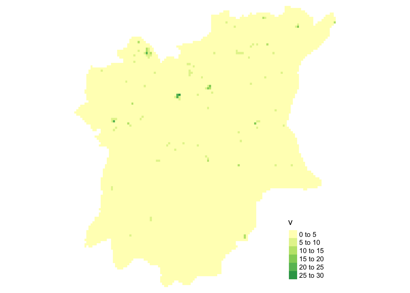
From the map above generated by kde_wp_functional_bw_raster, we can see that there are not many functional water points in Osun State, Nigeria. Most of the functional water points are located in the left Northern parts of Osun State.
tm_shape(kde_wp_nonfunctional_bw_raster) +
tm_raster("v") +
tm_layout(legend.position = c("right", "bottom"), frame = FALSE)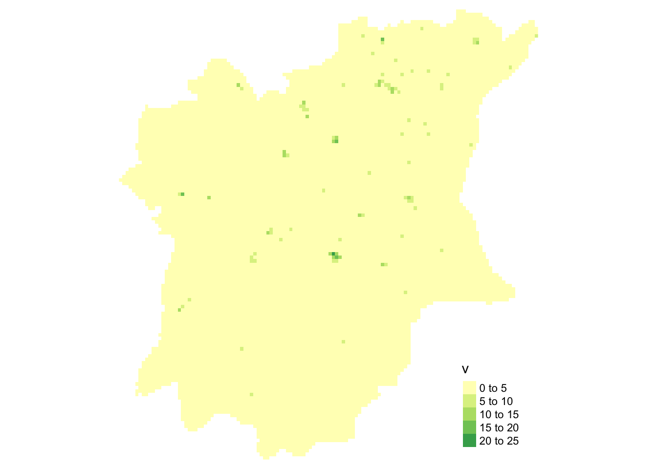
From the map above generated by kde_wp_nonfunctional_bw_raster, we can see that there are many non-functional water points in Osun State, Nigeria. Most of the non-functional water points are located in the right Northern parts of Osun State.
9.0 Spatial patterns revealed by the kernel density maps.
Most of the functional water points are located in the left Northern parts of Osun State. Most of the non-functional water points are located in the right Northern parts of Osun State.
10.0 Highlight the advantage of kernel density map over point map.
So, why use a kernel density map over the point maps? Let’s focus on the comparison below.
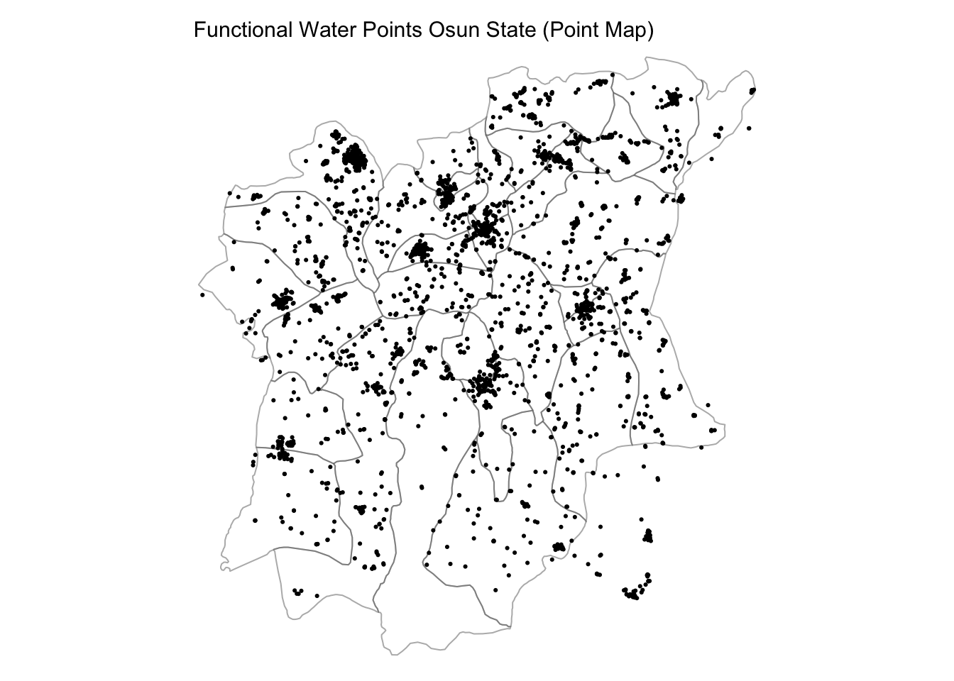
With the kernel density map, denser areas with a heavier distribution of functional/ non-functional water points in Osun State are easily spotted. The kernel density map uses a range of colours to indicate varying concentration levels.
However, for point maps, the points are scattered over the map without varying colours to indicate different concentration levels.
As such, it would require more effort to locate different regions of different concentrations from a point map than it would from a kernel density map.
11.0 Second-order Spatial Point Patterns Analysis
To confirm the observed spatial patterns above, a hypothesis test will be done.
11.1 Hypothesis Test: Functional Waterpoints in Osun State Random Distribution
The hypothesis and test are as follows:
Ho = The distribution of functional waterpoints in Osun State, Nigeria are randomly distributed.
H1= The distribution of functional waterpoints in Osun State, Nigeria are not randomly distributed.
Significance level: 95%
The null hypothesis will be rejected if p-value is smaller than alpha value of 0.05.
In this section, you will learn how to compute L-function estimation by using Lest() of spatstat package. You will also learn how to perform monta carlo simulation test using envelope() of spatstat package.
L_waterpoint_func = Lest(wp_functional_osun_ppp, correction = "Ripley")
plot(L_waterpoint_func, . -r ~ r,
ylab= "L(d)-r", xlab = "d(m)")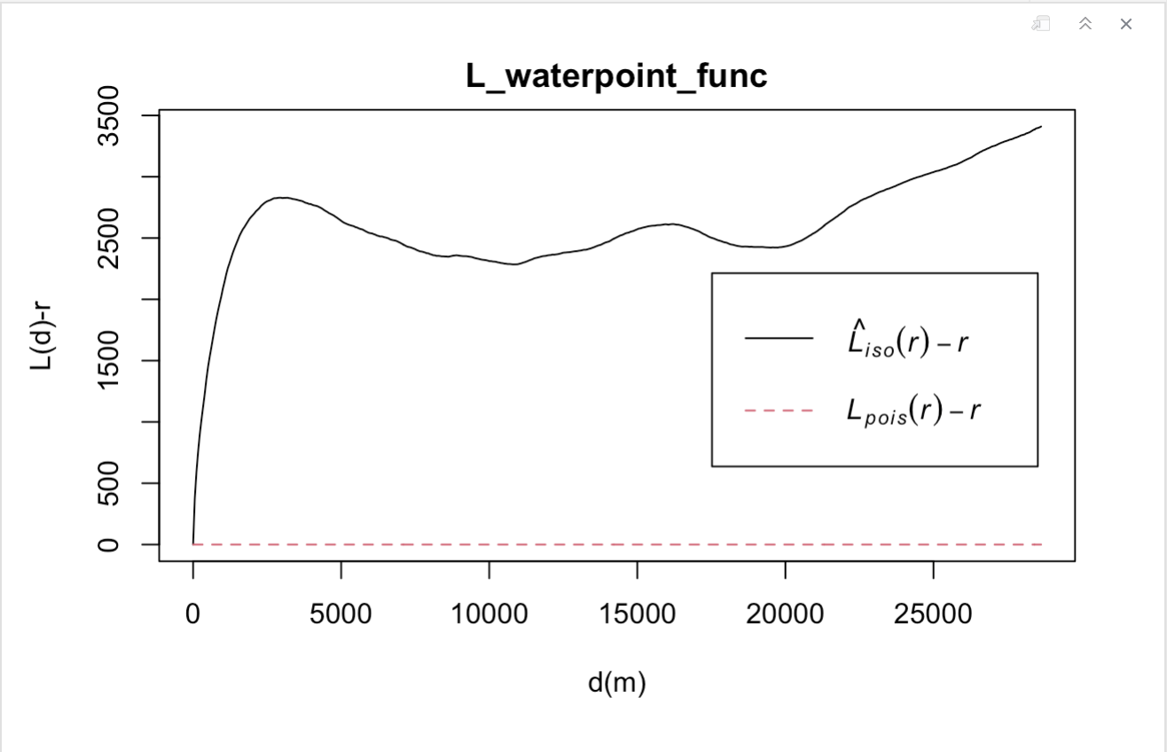
11.1.1 Performing Complete Spatial Randomness Test
L_waterpoint_func.csr <- envelope(wp_functional_osun_ppp, Lest, nsim = 39, rank = 1, glocal=TRUE)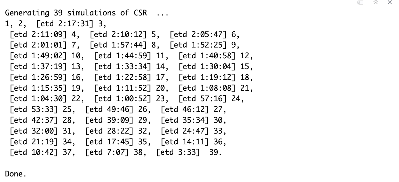
plot(L_waterpoint_func.csr, . - r ~ r, xlab="d", ylab="L(d)-r")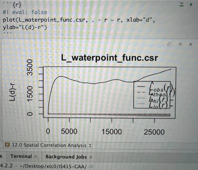
This picture was used instead as I misplaced my screenshot and could not rerun this in time. However, I actually did run this cell as seen from the picture’s GitHub username. It’s the same GitHub username used in my Netlify link.
11.1.2 Analysis Obtained
As the L value is greater than its corresponding L(theo) value for all distances, the observed distribution for functional water points in Osun State, Nigeria is geographically concentrated. The L value is above the upper confidence envelop too. The spatial clustering of functional water points observed is statistically significant. At 95% significance level, we reject the null hypothesis which states that the distribution of functional waterpoints in Osun State, Nigeria are randomly distributed.
This means that the functional waterpoints in Osun State, Nigeria are NOT randomly distributed.
11.2 Hypothesis Test: Non-Functional Waterpoints in Osun State Random Distribution
The hypothesis and test are as follows:
Ho = The distribution of non-functional waterpoints in Osun State, Nigeria are randomly distributed.
H1= The distribution of non-functional waterpoints in Osun State, Nigeria are not randomly distributed.
Significance level: 95%
The null hypothesis will be rejected if p-value is smaller than alpha value of 0.05.
L_waterpoint_nonfunc = Lest(wp_nonfunctional_osun_ppp, correction = "Ripley")
plot(L_waterpoint_nonfunc, . -r ~ r,
ylab= "L(d)-r", xlab = "d(m)")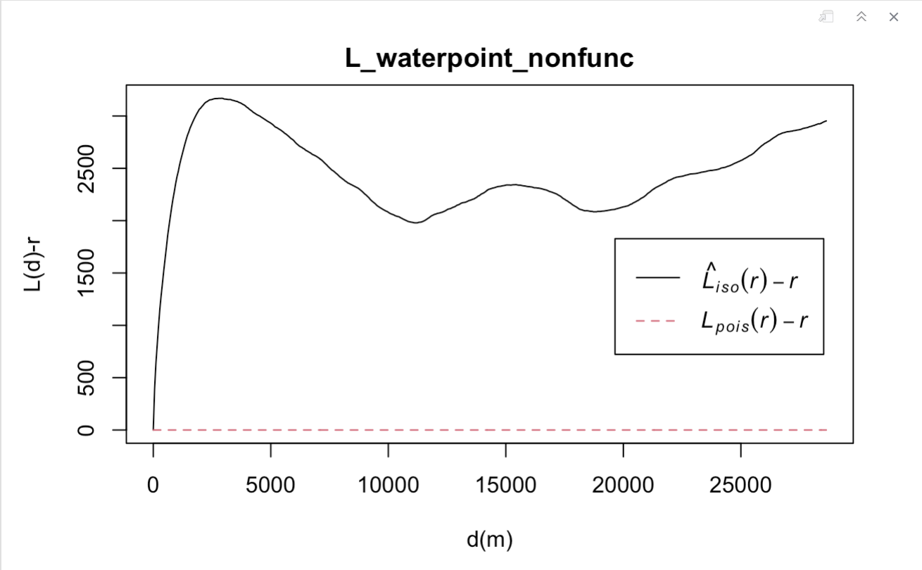
11.2.1 Performing Complete Spatial Randomness Test
L_waterpoint_nonfunc.csr <- envelope(wp_nonfunctional_osun_ppp, Lest, nsim = 39, rank = 1, glocal=TRUE)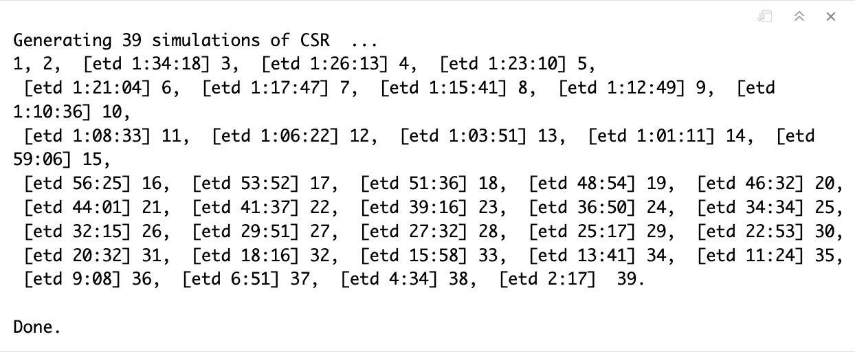
plot(L_waterpoint_nonfunc.csr, . - r ~ r, xlab="d", ylab="L(d)-r")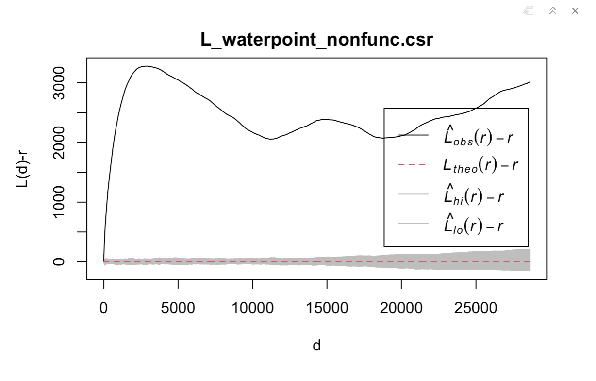
11.2.2 Analysis Obtained
As the L value is greater than its corresponding L(theo) value for all distances, the observed distribution for non-functional water points in Osun State, Nigeria is geographically concentrated. The L value is above the upper confidence envelop too. The spatial clustering of non-functional water points observed is statistically significant. At 95% significance level, we reject the null hypothesis which states that the distribution of non-functional water points in Osun State, Nigeria are randomly distributed.
This means that the non-functional waterpoints in Osun State, Nigeria are NOT randomly distributed.
12.0 Spatial Correlation Analysis
The hypothesis and test are as follows:
Ho = The spatial distribution of functional and non-functional waterpoints in Osun State, Nigeria are independent from each other.
H1= The spatial distribution of functional and non-functional waterpoints in Osun State, Nigeria are not independent from each other.
Significance level: 95%
The null hypothesis will be rejected if p-value is smaller than alpha value of 0.05.
12.1 Local Colocation Quotients (LCLQ)
pacman::p_load(sfdep)We will perform local colocation quotient analysis to determine if the spatial distribution of functional and non-functional water points are independent from each other.
In order to use the local_colocation(A, B, nb, wt, 49) function, we would need to gather the parameters first.
To get the nb parameter value, we will need to get the sf dataframe of all waterpoints in Osun State, Nigeria.
func_nonfunc_wp <- wp_sf_nga %>%
filter(status_clean %in%
c("Functional",
"Functional but not in use",
"Functional but needs repair",
"Abandoned/Decommissioned",
"Abandoned",
"Non-Functional due to dry season",
"Non-Functional",
"Non functional due to dry season"))func_nonfunc_wpSimple feature collection with 4809 features and 1 field
Geometry type: POINT
Dimension: XY
Bounding box: xmin: 177285.9 ymin: 340054.1 xmax: 290751 ymax: 450859.7
Projected CRS: Minna / Nigeria Mid Belt
# A tibble: 4,809 × 2
status_clean Geometry
* <chr> <POINT [m]>
1 Abandoned/Decommissioned (260303.8 368418.2)
2 Abandoned/Decommissioned (236239.7 417577)
3 Abandoned/Decommissioned (244631.9 447614.1)
4 Abandoned/Decommissioned (252887.8 432017.8)
5 Abandoned/Decommissioned (202912.5 390196.1)
6 Functional but needs repair (212810 386707.6)
7 Functional (228798.9 403822.5)
8 Functional (270497.9 377476.9)
9 Functional (212202 349210.1)
10 Functional (259331.9 399591.4)
# … with 4,799 more rowsNow, we can pass in the func_nonfunc_wp sf dataframe into the include_self() function to get the nb parameter value.
nb <- include_self(
st_knn(st_geometry(func_nonfunc_wp), 6)
)We will proceed to find wt parameter value.
wt <- st_kernel_weights(nb,
func_nonfunc_wp,
"gaussian",
adaptive = TRUE)We will now assign the A parameter a value. The A parameter is the target.
A <- wp_functional$status_cleanB parameter is the neighbour we want to know if A is co-located with and if so, to what extent.
B <- wp_nonfunctional$status_cleanNow, we’ll put all the parameters into the local_colocation function.
LCLQ <- local_colocation(A, B, nb, wt, 49)LCLQ_wp <- cbind(func_nonfunc_wp, LCLQ)tmap_mode("view")
tm_shape(osunNGA) +
tm_polygons() +
tm_shape(LCLQ_wp) +
tm_dots(col = "Non.Functional",
size = 0.01,
border.col = "black",
border.lwd = 0.5) +
tm_view(set.zoom.limits = c(9,16))tmap_mode("view")
tm_shape(osunNGA) +
tm_polygons() +
tm_shape(LCLQ_wp) +
tm_dots(col = "p_sim_Non.Functional",
size = 0.01,
border.col = "black",
border.lwd = 0.5) +
tm_view(set.zoom.limits = c(9,16))# return tmap mode to plot for future visualisations
tmap_mode("plot")12.2 Local Colocation Quotients (LCLQ) Statistical Conclusions
We can tell that in some functional water point regions of Osun State, where the colocation quotient is > 1 (as indicated by dark orange and red spots), we can see that there’s a high likelihood that the non-functional water points exist nearby in the region.
For functional water point regions where colocation quotient is < 1 (as indicated by colours lighter than light orange), we can see that there’s a low likelihood that non-functional water points exist nearby in the region.
For functional water point regions where colocation quotient is = 1 (as indicated by orange spots), we can see that there’s a good mix of both functional and non-functional water points in the region.
We can see that non-functional water points aren’t as prevalent as functional water points in Osun State.
There are stronger signs of colocation between functional and non-functional waterpoints towards the leftmost and rightmost regions of Osun State. However for the majority of Osun State, the functional water points have no colocation with non-functional water points.
Moreover, there are NOT many regions on the map that shows a low p-value (smaller than 0.05). As such, at 95% confidence level, there’s not sufficient evidence to reject the null hypothesis which states that the spatial distribution of functional and non-functional waterpoints in Osun State, Nigeria are independent from each other.
We continue to conclude that the spatial distribution of functional and non-functional waterpoints in Osun State, Nigeria are independent from each other.